[Update: Edited significantly on 8 November 2008 to include results from TreeTagger and MorphAdorner. Tables reworked and discussion and conclusions modified. For a full list and discussion of the packages under review, see “Evaluating POS Taggers: The Contenders“; the background info on Lingpipe and the Stanford tagger that previously was here has been moved to that post.]

[Update 2: Added results from Joyce rerun.]

[Update 3: See Bob Carpenter’s (of alias-i, the author and all-around guru of LingPipe) very helpful comment below for a list of things that have a potentially significant impact on speed, both for LingPipe and for the other taggers. These numbers are to be taken with a significant grain of salt in light thereof. Thanks, Bob!]

The part-of-speech taggers I’m evaluating are MorphAdorner, Lingpipe, TreeTagger, and the Stanford Log-Linear POS Tagger (one of these kids: not named like the others). See the link in the update note above for all the details.

Test setup

I’m using a dual-core Athlon 64 X2 3600+ system with two GB RAM running 64-bit Fedora 9. The machine is a desktop, and it’s a couple of years old; it’s not the fastest thing around, but neither is it especially slow. The JRE is Sun’s 64-bit package, version 1.6.0_10 (the latest release at the time of writing).

Tagging is an easily parrallelized task, and this is a dual-core system, but I didn’t take any steps to make use of this fact; in general, the taggers used 100% CPU time on one core and a smaller amount of time (1%-30%) on the other. It would be great if there were a simple way to tell Java to use both cores fully, but if there is, I haven’t come across it. For larger jobs, I would write a simple batch job to start as many Java instances as there are cores (but note that total system memory requirements could be an issue in that case; hello, Newegg!).

The taggers were invoked using the following commands, with all variables defined as appropriate. (This section is pretty skippable unless you want to repeat my tests. The short version: I gave Java about a gig of RAM and looped over the input files with a simple for loop unless there was an explicit option to process an entire input directory. There are also some notes on specific options used with each package.)

Lingpipe

For Lingpipe running over individual files:

for i in $( find $inputDir -printf "%P\n" ); do
   /usr/bin/time -a -o $logFile \
      ./cmd_pos_en_general_brown.sh \
      -resultType=firstBest -inFile=$inputDir/$i \
      -outFile=$outputDir/$i >> $logFile 2>&1
done

Note that in this and all other commands, I’m timing the runs with /usr/bin/time. This could—and would—obviously be left out if I weren’t benchmarking.

For Lingpipe running over entire directories the command was the same, but without the for loop and with -*Dir in place of the corresponding -*File options.

The main thing to note is that I’m using the generic tagger trained on the Brown corpus (supplied with the Lingpipe distribution) and am using “first best” results rather than n-best or confidence-weighted listings for each word/token (which are roughly 1.5 and 2.5 times slower, respectively). The differences between the result types are explained in Lingpipe’s POS tutorial; the short version is that first-best gives you the single best guess at each word’s part of speech, which is all I’m looking for at the moment. I do think it would be interesting in the long run, though, to see what kinds of words and situations result in high-confidence output and which are confusing or marginal for the tagger.

Stanford

For Stanford, the command line is:

for i in $( find $inputDir -printf "%P\n" ); do
   /usr/bin/time -a -o $logFile java -mx1g \
      -classpath stanford-postagger.jar \
      edu.stanford.nlp.tagger.maxent.MaxentTagger \
      -model models/$modelType -textFile $inputDir/$i \
      > $outputDir/$i
done

$modelType is either bidirectional-wsj-0-18.tagger (“bidirectional”) or left3words-wsj-0-18.tagger (“left3”). As invoked, the tagger produces plain-text output, though it can be set to use XML (I think; I know this is true with XML input, but my brief attempt to get XML output didn’t work. Will investigate further if necessary).

MorphAdorner

The MorphAdorner command line to loop over individual files in a directory is:

for i in $( find $inputDir -printf "%P\n" ); do
   /usr/bin/time -a -o $logFile ./adornplaintext \
      $outputDir $inputDir/$i >> $logFile 2>&1
done

This is fine (I do like those for loops), but it could be better. MorphAdorner doesn’t appear to have a direct way to specify an input directory rather than individual files, but it’s happy to take wildcards, which has the same effect and is much faster than the loop version above (because it doesn’t have to load lexical data over and over again). This is then surely the preferred form:

/usr/bin/time -a -o $logFile ./adornplaintext $outputDir \
   $inputDir/\*.txt >> $logFile 2>&1

Note that I have—following a certain amount of headbanging, because I’m an idiot—escaped the wildcard. adornplaintext is a simple script to invoke the Java processor with the appropriate settings; it’s supplied with the distribution and uses the NCF (nineteenth-century British fiction, mostly) training data. The only change I made was to raise the max Java heap size to 1440m, since the default 720m threw errors on a couple of the larger texts.

TreeTagger

TreeTagger, unlike the other three, isn’t a Java program, so there’s no mucking about with Java parameters. Otherwise, it looks similar. (None of this is rocket science, of course; it’s all just here for documentation.)

for i in $( find $inputDir -printf "%P\n" ); do
   /usr/bin/time -a -o $logFile ./tree-tagger-english \
      $inputDir/$i > $outputDir/$i
done

Same story as most of the others with the lack of an input directory option, but the overhead penalty is much smaller with TreeTagger, so I made no attempt to work around it. tree-tagger-english is, again like many of the others, a small script that sets options and invokes the tagging binaries. I left the defaults alone.

Further Notes

The small archive of texts I’m using to benchmark is described in my previous post. Just for recall: Fourteen novels, 2.4 million words.

I ran each of the taggers over the archive three times and took the average time required to process each text (or directory). Stanford bidirectional was too slow for multiple runs, so it was run only once. There were no significant outlying times for any of the texts in any of the runs, i.e., there was no immediate reason to be suspicious of this simple time averaging.

Results

First, a list of the elapsed times, in seconds, for the various taggers and models.

(Apologies for lack of monospaced fonts in the tables, which seems to be a wordpress.com issue. I should also probably reorder tables 1 and 2, but that would be a pain in the hand-coded HTML ass.)

Key
LP = Lingpipe
SL = Stanford, left3words model
SB = Stanford, bidirectional model
TT = TreeTagger
MA = MorphAdorner

Table 1: Run times

All times in CPU seconds, measured from the output of /usr/bin/time, summing user and system CPU time, not wall clock time. Word counts from wc -w for consistency; most taggers measure tokens (including punctuation) rather than words, so their internal word counts are higher than the figures listed here and are not mutually consistent. Lower numbers are better.

Author	Words	LP	SL	SB	TT	MA
Alcott	185890	34	468	13582	9	132
Austen	118572	21	214	4319	9	105
Brontë	185455	32	495	17452	9	127
Conrad	38109	10	104	2824	2	85
Defoe	121515	20	205	4552	5	112
Dickens	184425	34	401	9587	9	128
Eliot	316158	56	807	29717*	14	170
Hawthorne	82910	18	280	8060	4	96
Joyce	264965	42	1791	95906*	12	177
Melville	212467	38	933	33330	10	139
Richardson	221252	41	414	11506	10	136
Scott	183104	34	740	27176	9	129
Stowe	180554	35	528	16264	9	129
Twain	110294	22	288	8778	5	111
Total:	2405670	437	7668	283054	112	1775
By dir:	2405670	323	—	—	—	593

“By dir” = tagger run over entire input directory rather than over individual files.

*Total times extrapolated from incomplete runs; tagger crashed with
Java out of memory error at 93% complete for Eliot and 43% for Joyce. The Eliot is close enough to use, I think, but the Joyce is dubious, especially since it’s such an outlier. See notes below. [Update: I just reran the Joyce using a gig and a half of memory for Java. Result: 227,708 seconds of CPU time. That’s more than two and a half days. Seriously. Whatever’s going on with this, it’s strange.]

Table 2: Speeds

Words tagged per CPU second. Higher is better.

Author	LP	SL	SB	TT	MA
Alcott	5429	397	13.7	19692	1412
Austen	5775	554	27.5	19828	1125
Brontë	5864	375	10.6	19570	1459
Conrad	3862	366	13.5	16862	449
Defoe	6146	592	26.7	20654	1090
Dickens	5479	459	19.2	19774	1436
Eliot	5673	392	10.6	20924	1860
Hawthorne	4595	296	10.3	19341	862
Joyce	6286	148	2.8*	19695	1501
Melville	5535	228	6.4	19685	1529
Richardson	5439	535	19.2	20274	1627
Scott	5341	247	6.7	19990	1424
Stowe	5103	342	11.1	18775	1396
Twain	4903	383	12.6	18736	994
Average:	5507	314	8.5*	19786	1335
By dir:	7443	—	—	—	4058

*If the dubious Joyce result is excluded, the average speed rises to 11.4 words per second. I’ve used this higher value in the speed comparisons below.

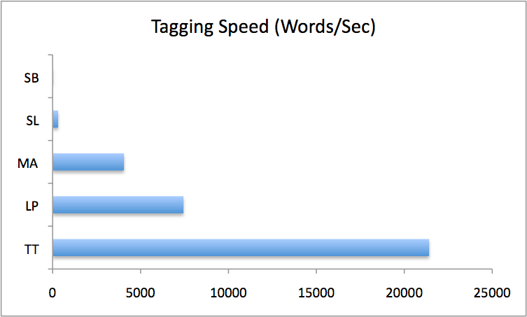
Table 3: Speed ratios

Ratio of words tagged per CPU second. Read as: Column entry over row entry, e.g., TreeTagger is 2.9 times faster than Lingpipe. Tagging speed in words per second added for reference.

Note that I’ve used the “by directory” speeds for Lingpipe and MorphAdorner, and excluded the possibly anomalous Joyce result from the Stanford bidirectional speed.

Type		TT	LP	MA	SL
	Speed	(21414)	(7443)	(4058)	(314)
LP	(7443)	2.9
MA	(4058)	5.3	1.8
SL	(314)	68	24	13
SB	(11.4)	1872	651	355	27

All of this in graphical form:

 

Discussion

The TreeTagger, Lingpipe, and Morphadorner taggers are all very fast; they process entire novels in seconds. Their speed is pretty consistent, too, though this fact is hidden a bit in the case of MorphAdorner by its significant startup overhead (20-30 seconds). Looking at MorphAdorner’s speed over the entire testing directory, rather than file by file, gives not only a much higher average speed (4000 wps vs. 1300) but much more consistent speed results (not shown in the tables above).

[Update: As noted above, cf. Bob Carpenter’s comment below for some notes on speed.]

These taggers tend to be slowest on the shortest works, especially Conrad, probably because there’s a fixed amount of overhead to start up a Java instance and perform another initialization steps, and Conrad’s novel is short enough for that to be a significant amount of the total processing time. This isn’t an issue in runs over an entire directory, where there’s only one startup instance, rather than file by file, and the overhead penalty in that case drops to zero as the corpus size becomes arbitrarily large.

Both Lingpipe and TreeTagger have the option to produce probabilistic results, that is, to produce output that includes several candidate parts of speech and the probability that each is correct for a given token. In Lingpipe, there’s a moderate penalty for doing so, somewhere around doubling the run time; in TreeTagger, the penalty is almost vanishingly small, around 10%.

Stanford’s tagger is much slower, working through novels in minutes or hours, depending on the analytical model used. There’s more variation in speed, too; the left3 model shows about a 4x difference between Joyce (slow) and Defoe (fast). Even excluding Joyce, which is something of an outlier, there’s a 2.6x difference between Melville and Defoe. The bidirectional model is similarly variable, especially if the Joyce result is correct. There’s a 10x spread between fastest and slowest results, or about 4x excluding Joyce.

The difference in tagging speed on Joyce in particular is interesting to me. Ulysses is surely the strangest and least conventionally grammatical of the bunch, and it doesn’t entirely surprise me that it should take longer to tag than the others. In fact I’m a bit suspicious of the fact that the other taggers not only don’t take longer to process it, but in some cases actually chew through it faster than any other text. Are they just throwing up their metaphorical hands and labeling a bunch of stuff junk? But I may be anthropomorphizing the algorithms. Just because I would find it hard to sort out Joyce doesn’t necessarily mean it’s especially hard to compute. Will look at this in the next post, on accuracy.

Comparing the taggers and models by speed, the TreeTagger, Lingpipe and MorphAdorner packages are all within an order of magnitude of one another. They are in turn one to two orders of magnitude faster than Stanford left3 and hundreds to thousands of times faster than Stanford bidirectional. Stanford left3 is about 30 times faster than Stanford bidi.

Conclusions

Everything here is provisional until I look at accuracy, obviously.

First, note that speed is a threshold property, as far as I’m concerned. Faster is better, but the question isn’t really “which tagger is fastest?” but “is it fast enough to do x” or “how can I use this tagger, given its speed?” I think there are three potentially relevant thresholds:

1. As a practical matter, can I run it once over the entire corpus?
2. Could I retag the corpus more or less on whim, if it were necessary or useful?
3. Could I retag the corpus in real time, on demand, if there turned out to be a reason to do so?

The first question is the most important one: I definitely have to be able to tag the entire corpus once. The others would be nice, especially #2, but I don’t yet have a compelling reason to require them.

With that in mind, there would have to be a pretty analytically significant difference in output quality to justify using the Stanford bidirectional tagger. Some quick calculations: Gutenberg has probably around 2500 usable English-language novels. Say they average 150,000 words each. Both of these are conservative estimates. That would mean 375 million words to tag. Assume, generously, that Stanford bidi averages 12 words per second. So a year of CPU time to tag the corpus. That could be cut down to something manageable with multiple, faster machines, but still, unless I get serious compute time, it would probably take a month or two. In principle, you only need to tag the dataset once, so this might be acceptable if it really did improve the analysis, but options 2 and 3 above would definitely be out with the bidi model, barring a major change in the amount of computing power at my disposal.

Also: The system requirements of the bidirectional model may be significant. As noted in passing above, giving Java a gig of RAM wasn’t enough for the Joyce and Eliot texts, which crashed out with insufficient memory at 43% and 93% complete, respectively. They’re too bloody slow to retest at the moment with 1.5 GB allocated. In any case, I couldn’t currently go above that, since I only have 2 gigs in the system. True, memory is cheap(ish), but it’s neither free nor infinite. A related point to investigate if necessary: Would more memory or other tweaks significantly improve speed with either of the the Stanford models?

The non-Stanford taggers could tag the entire corpus in a CPU day or less, and perhaps as little as an hour or two of real time with a small cluster. That would allow a lot of flexibility to rerun and to test things out. Stanford’s left3 model would take about two CPU weeks. That’s not ideal, but it’s certainly a possibility.

None of the taggers looks fast enough to do real-time reprocessing of the entire corpus given current computational power, but they could easily retag subsections in seconds to minutes, depending on size.

Finally, a brief foretaste on accuracy: Stanford’s own cross-validation indicates that the bidirectional model is 97.18% accurate, while left3 is 96.97%. It’s hard to imagine that 0.21% difference being significant, especially when both models drop to around 90% on unknown words. Haven’t yet seen or run similar tests on the others, nor have I done my own with Stanford. There’s reason to believe that MorphAdorner will be especially good on my corpus, given its literary training set, but that has yet to be verified; training other taggers on MorphAdorner’s data might also be possible.

Takeaway points on speed

Provisionally, then: MorphAdorner is probably the frontrunner: It’s fast enough, free, under current development, and geared toward literature. TreeTagger is fastest, but not by a qualitative margin. I’m also concerned that it’s not currently being developed and that the source code doesn’t appear to be available. Lingpipe is plenty fast, though I have some concerns about the license. Stanford left3 remains viable, but speed is a moderate strike against it. Stanford bidirectional is likely out of the running.