After a couple days off, I’ve been trying to run cross-validation on the Stanford tagger. The good news is that it works, more or less; I can feed training data to it and get a trained model out, which I can then use to tag new text. The bad news is that the training process keeps crashing out of memory (given 3800 MB to work with) on data sets over about 1M words. I emailed the helpful folks at Stanford, who pointed out that my training data (from MorphAdorner), in addition to being significantly larger than what they normally use (about 4M words instead of 1M; 500+ word maximum sentence length instead of about half that), was using 420+ tags, which made training impossible under 4GB of physical memory.

420 tags was news to me; NUPOS contains about 180 valid tags. So I wrote a little script to list the tags used in the training data, and immediately discovered the problem. Recall that MorphAdorner training data usually looks like this:

Her     po31    she     her
mother  n1      mother  mother
had     vhd     have    had
died    vvn     die     died
too     av      too     too
long    av-j    long    long
ago     av      ago     ago
[...]

One word, one tag, one lemma, one standard spelling. As I’ve noted before, it also passes punctuation unmodified, like this:

,       ,       ,       ,

or

*****   *****   *****   *****

Not all such punctuation is part of the standard NUPOS tagset, of course (for the record, the only punctuation included in the “official” NUPOS tagset is “. ; ( ) ,”). So some of the extra tags in the training data are simply funky punctuation. But that doesn’t explain all (or even most) of the discrepancy (there are maybe 30-40 unique instances of such punctuation in the training data).

So what gives? Turns out that MorphAdorner does something clever with contractions: it treats them as two words in one, and gives them two tags on a single input line. A couple of examples:

done's  vvn|vbz    done|be done's
off's   a-acp|po31 off|he  off's

Note the “|” separator. I can’t remember if I’d noticed this before (it occurs about 22K times in 4M lines of training data, so it wouldn’t necessarily jump out in a visual inspection), but in any case I definitely didn’t do anything about it when I fed the training data to TreeTagger or Stanford. This surely accounts for some of the abysmal accuracy results I saw with TreeTagger, and it’s a major culprit in my memory woes with Stanford. It adds 197 items that look like tags to Stanford, roughly doubling the tagset size, and since the training process involves a two-dimensional array of tags, it therefore roughly quadruples the memory requirements. Coincidentally, that happens to be about the difference in size between the full training dataset (3.8M words) and the largest sample I’ve used successfully to train Stanford (1M words).

The good news is that it’s probably largely fixable with some data munging. If I were maximally lazy, I could just kill all the lines in question. Or I could split them in two at the apostrophe and the vertical bar in their respective fields. Either way, relevant information would be lost and output quality would presumably drop, though not so much as at the moment, when I’m feeding the Stanford tagger what is effectively bad data. I’ll try the simple deletion method first, just to see if it allows me to run the trainer on a data set this large, then worry about handling things properly later.

[Update: Martin Mueller fills me in via email concerning the use of compound tags in the MorphAdorner training data:

So the compound tags are in a very real sense “true” single tags that just happen to be made up of two otherwise-valid individual tags. The 423 tags in the MorphAdorner training data are thus to be treated as 423 unique features/tag-types, or at least that’s how MorphAdorner does it. This doesn’t solve my memory-use problem, but it’s good to know.
]

More on TreeTagger, which I’ve now (finally) gotten to train and cross-validate.

First, a note on an additional difficulty not included in the last post. I use MorphAdorner to create the lexicon from each chunk of training data (once that data has been cleaned up to TreeTagger’s liking). This works well, except that MorphAdorner has a quirk in its handling of punctuation for the lexicon. Specifically, MorphAdorner treats left and right quotes, which are tagged in the training data with ‘lq’ and ‘rq,’ as punctuation to be passed through in the lexicon. So what appears in the training data like this (sic, incidentally, on the “ here):

“	lq	“

appears in the lexicon as:

“	“	“

I think there’s a way to fiddle with smart quotes in MorphAdorner (it would be nice to treat them all as dumb double or single quotes, though maybe MorphAdporner’s clever enough to use left and right quotes for context info), but I can’t find it at the moment. Anyway, this freaks TreeTagger out. So I’ve modified my fix-everything-up-for-TreeTagger script to change the second form into the first whenever left or right quotes appear in the lexicon. Meh.

Results and Discussion

All that said, and two days of my life that I’ll never get back squandered, was it at least worth it? In a word: No. TreeTagger produces awful results in the cross-validation tests. See for yourself:

#       Words   Errors   Err Rate
0       382889  58934   .153919
1       382888  57586   .150399
2       382888  52527   .137186
3       382889  51714   .135062
4       382888  45794   .119601
5       382888  44436   .116054
6       382889  54037   .141129
7       382888  55332   .144512
8       382888  52674   .137570
9       382888  52441   .136961
Tot    3828883 525475   .137239

Recall that for MorphAdorner the average error rate in cross-validation was 2.3-2.9%, depending on the lexical data used. Here it’s 13.7%. This is obviously totally unusable. And a quick survey of the data suggests that the errors are neither easily systematic nor trivial—there are nouns tagged as verbs and such all over the place.

[A side note: TreeTagger doesn’t show the disparity on the Shakespeare-heavy tranches, nos. 6-8, that MorphAdorner did. But the error rates are so high that it’s hard to say anything more about it. I hope to look at those chunks again in the Stanford case.]

It’s possible—likely, even—that I’ve done something wrong, given how bad the results are. TreeTagger’s authors claim to have achieved 96+% accuracy on general data using a smaller tagset. It’s also surely true that the tagset and cardinal/ordinal restrictions on TreeTagger’s training input limit its accuracy in the present case. Whatever. I’m sick of dealing with it.

[Update: Some of the errors are surely due to my not having reworked the training data to set a sentence-end tag the way TreeTagger expects. (I used ‘.’ instead—close, but of course not perfect.) But that would account for only a small fraction of the total errors, and to fix it at this point would require more work than I’m will to spend on a solution that obviously won’t beat MorphAdorner.]

Out of curiosity, I’ll still run TreeTagger through the stock-training-data-and-reduced-tagset comparison of all the taggers that will be the last test in this roundup, but for now TreeTagger’s very likely out of the running, especially since I’d like to have NUPOS compatibility.

As always, things aren’t as easy as it seems they should be. Specifically, TreeTagger—which looked like it was going to be very easy to retrain, hence also easy-ish to cross-validate—turns out to be mildly tricky. Tricky enough that I’m sick of dealing with it.

Why It Looks Easy

To train TreeTagger, you supply it with a lexicon (word, POS tag, lemma, plus additional POS-lemma pairs for words that can function as multiple parts of speech), a list of valid tags, a tab-delimited training file (again, word-POS-lemma), and a “sentence-end” tag (which replaces the POS tag for punctuation that ends a sentence; “SENT” by default). I have all of that data, except for the sentence-end tags (MorphAdorner tags punctuation as the mark itself, e.g., ‘!’ is tagged ‘!’ usw., with no differentiation of sentence ends/breaks). But the SENT tag is configurable, and I could probably fudge by setting it to ‘.’.

Why It Isn’t

The main problem is that TreeTagger insists that the tags used in the supplied tagset match exactly those used in the training data and in the lexical data, which (training and lex tags) must in turn match each other. “Well, duh,” you say, “it can only know how to use tags you tell it about.” True, but here’s the thing: It chokes on extra tags in the tagset or the lexicon, not just in the training data. So you can’t use one tagset or lexicon for all the training; you have to custom-generate a lexicon and a list of tags for every training set you want to use. You’d want to custom-generate the lexicon anyway, though it would be nice to be able to test against the enhanced lexicon supplied with MorphAdorner.

And then there’s the fact that, per the documentation, TreeTagger shouldn’t be trained or cardinal and ordinal numbers that contain digits, so you need to strip them from the training and lexical data, but keep them in cases where they’re spelled out. Plus, as mentioned above, MorphAdorner doesn’t have a generic punctuation tag—it passes punctuation through, tagged as the punctuation itself. And it groups adjacent punctuation marks together, most noticeably blocks of periods ‘…’, ‘..’, ‘…..’, etc. But chunks of random punctuation are of course not valid NUPOS tags, so you don’t really want them in the training or tag sets.

So here’s what would be required to run cross-validation, as far as I can tell, above and beyond the data-chunking-and-stripping scripts that I already have: A script that iterates line-by-line over the training data (recall: formatted “word-POS-lemma[-pos-lemma[-pos-lemma…]],” where the extra POS-lemma pairs are occasional features of which there may be arbitrarily many), removing lines that have a digit in the word and a POS tag of “crd” or “ord”, unless they also have another POS tag, in which case only the offending POS-lemma pair should be removed; removes any line with a POS tag not in the full NUPOS set (in order to catch the multiple-punctuation business, plus any oddness that might have slipped into the training data by mistake; then adds the (now guaranteed to be valid) POS tags from the line to an array (or probably a hash) of valid-and-existant tags in this particular training set, checking to make sure the tag it’s adding isn’t a duplicate. And then regenerates the lexicon based on the resulting, reduced training set.

And at that point it should be possible to train TreeTagger on MorphAdorner’s data, hence to cross-validate it. Maybe. Unless I’ve missed something. Which is likely.

I’m going to spend a few (more) hours banging my head against this, but only to the end of the day today, tops.

“Damn,” you may be saying, “is he still on about this stuff?” Yes, yes I am.

So … MorphAdorner is easy to retrain/validate, because I have access to the tagged, formatted training data. This is what I reported in my previous post on cross-validation.

Now I want to see how much work would be involved in trying to train the other taggers on MorphAdorner’s data. I’m interested in doing this because MorphAdorner is the only one of the bunch that’s trained on literary texts rather than general contemporary sources (often a standard corpus from the 1989 Wall Street Journal). If it’s easy enough, I’ll retrain any/all of the other taggers to see if they produce better results (and if so, how much better) before I compare them to MorphAdorner.

A related note: It will be especially nifty if the other taggers can use an arbitrary tagset. Or, well, not arbitrary. NUPOS. NUPOS is good, for reasons mentioned earlier. Plus, that would make direct use of the MorphAdorner training data much easier, and it would make a direct comparison of outputs easier as well. If this tagset agnosticism isn’t built into the other taggers, I’ll have to convert between tagsets.

The rest of this post, then, is my notes on what’s involved in training the other taggers, with an eye specifically toward using MorphAdorner’s data/tagset.

The MorphAdorner Training Data

The training data I have from MorphAdorner has a pretty simple four-column, tab-delimited format. It’s just word pos-tag lemma std-spelling. And sentences are followed by a blank line, which makes it easy to pick them out if necessary. A snippet:

She     pns31   she     she
had     vhd     have    had
always  av      always  always
wanted  vvn     want    wanted
to      pc-acp  to      to
do      vdi     do      do
[...]

So it should be pretty easy to transform it into whatever (text-based) form might be required for the other taggers.

LingPipe

LingPipe is a bit of a problem. To train it on a new corpus, I’d need to write a moderate amount of Java code, plus munge the training data a bit. There are examples provided for analogous cases (assuming proper input), and the documentation is good, but this would probably be a week-long project. I’d be willing to invest that amount of time if I had reason to believe the results would be superior, but here’s the thing: LingPipe uses a Hidden Markov Model, as does MorphAdorner. It’s not that much faster than MorphAdorner (about 2x, but that’s likely to drop over a larger corpus, since MorphAdorner has higher one-time startup overhead than LingPipe). And it’s licensed in a way that probably makes it unusable with nonredistributable corpora. So do I want to send a week, however edifying it might be, evaluating whether or not LingPipe might be meaningfully superior to MorphAdorner, when there’s good reason to expect that it will not be? I’m going with no.

What I will do, though, is compare its default output (using the Brown training data) to MorphAdorner’s over the training corpus to get a sense of its accuracy using the built-in model(s). That’s just a matter of working up a set of translations between NUPOS and LingPipe’s tagsets, plus some XML-munging Perl-fu.

Stanford

Stanford looks easier, and it’s a more interesting case, since it uses a different algorithm (maximum entropy rather than Hidden Markov). Just need to transform the training data into the expected form and have at it. (Incidentally, maybe I can just set the tag delimiter to [tab]? Trivial, but investigate.) If this turns out to be as easy as expected (ha!), will run full cross-validation. All this probably using left3words only. I want no further part of the slow-as-molases-in-January bidirectional version, though I suppose I should look into it for the sake of completeness.

As above, I’ll also compare the retrained results to those already obtained using default training data.

TreeTagger

This also looks very easy to train using MorphAdorner’s data, so expect the same cross-validation and default comparisons.

Action Items

OK, so Stanford and TreeTagger will get full retraining and cross-validation (as MorphAdorner did before them), plus comparison of their default output to retrained cases. LingPipe will get only the latter.

Will write up (briefly) what’s involved in doing the retraining as I get into it. More in the next couple of days as results are available.

Here are the results of the cross-validation trials with MorphAdorner. Note to self: Never claim that anything will be trivial.

I ran a ten-fold cross-validation trial on the MorphAdorner training data. All fairly straightforward and naïve; I chopped the training data into ten equal-size chunks (with no attention to sentence or paragraph boundaries, which introduces edge cases, but they’re trivial compared to the sample size), trained the tagger on nine of them and ran it over the remaining one using the new training set, then repeated the process for each chunk. I did this in two forms: Once creating new lexical data as well as a new transformation matrix (columns labeled “1” below), and then a second time creating only a new transformation matrix, but using the supplied lexical information (labeled “2”). The true error rate on new texts is probably somewhere between the two, but (I think) likely to be closer to the second (better) case.

Results

So … the results:

#     Wds     Err1   Rate1    Err2    Rate2   Diff12   Rate12
0    382889   8607  .022479   7049   .018410   2143   .005596
1    382888   8267  .021591   5907   .015427   3120   .008148
2    382888   8749  .022850   6698   .017493   2739   .007153
3    382889   8780  .022930   7322   .019123   2168   .005662
4    382888   8039  .020995   5784   .015106   2851   .007446
5    382888   8147  .021277   5835   .015239   3020   .007887
6    382889  19660  .051346  16727   .043686   3721   .009718
7    382888  20494  .053524  17723   .046287   3679   .009608
8    382888  17078  .044603  14441   .037715   3603   .009410
9    382888   7151  .018676   4512   .011784   4436   .011585
Tot 3828883 114972  .030027  91998   .024027  31480   .008221

Key

# = Chunk being evaluated
Wds = Number of words in that chunk
Err1 = Number of tagging errors in the testing chunk using lexical and matrix data derived exclusively from the other cross-validation chunks
Rate1 = Tagging error rate for the testing chunk using this training data (1)
Err2 = Number of tagging errors using a matrix derived from the other chunks, but stock lexical data from the MorphAdorner distribution
Rate2 = Error rate in the second case
Diff12 = Number of differences between the output files generated by cases 1 and 2
Rate12 = Rate of differences between output 1 and 2

[Update: In my original test (the data reported above), I didn’t preserve empty lines in the training and testing data. Rerunning the cross-validation with empty lines in place produces very slightly better results, with overall average error rates dropping from 3.0% to 2.9% (using limited lexical data, case 1) and from 2.4% to 2.3% (with full lexical data, case 2). Rates corrected in the analysis sections below. Corrected data (where blank lines now count as “words”):

#     Wds     Err1   Rate1    Err2    Rate2   Diff12   Rate12
0    399644   8599  .021516   7045   .017628   2142   .005359
1    399643   8140  .020368   5886   .014728   3015   .007544
2    399643   8803  .022027   6737   .016857   2769   .006928
3    399644   8806  .022034   7347   .018383   2173   .005437
4    399643   8070  .020193   5817   .014555   2843   .007113
5    399643   8817  .022062   5918   .014808   3676   .009198
6    399644  19806  .049559  16901   .042290   3727   .009325
7    399643  20246  .050660  17486   .043754   3645   .009120
8    399643  16997  .042530  14362   .035937   3597   .009000
9    399643   7150  .017890   4512   .011290   4438   .011104
Tot 3996433 115434  .028884  92011   .023023  32025   .008013

]

Notes

A couple of observations. In general, the tagging quality is quite good; it averages 97.1% accuracy over the full testing set even when it’s working without the enhanced lexicon supplied with the distribution, and rises to 97.7% with it.

There’s some serious variability, especially in chunks 6, 7, and 8. A quick inspection suggests that they’re mostly Shakespeare, which I guess is both reassuring and unsurprising. Reassuring because I’ll mostly be working with later stuff and with fiction rather than drama; and unsurprising particularly in the case of cross-validation, since much of the Shakespeare is necessarily excluded from the training data when it happens to occur in the chunk under consideration. Without the Shakespeare-heavy chunks, accuracy is around 97.8% and 98.4% for cases 1 and 2, respectively. That’s darn good.

I don’t know what, if anything, to make of the difference rate between the two testing samples, which is quite small (less than 1%) but not zero. I guess it’s good to know that different training inputs do in fact produce different outputs. Note also the difference between them is not identical to the sum of the differences between each output and the reference data, i.e., it’s not the case that they agree on everything but the errors. Each case gets some words right that the other one misses. No surprise there.

This is all very encouraging; accuracy at 97% and above is excellent. And this is comparing exact matches using a very large tagset; accuracy would be even better with less rigorous matching. As a practical matter, I probably won’t be able to do equivalent cross-validation for the other taggers (too time consuming, even if it’s technically possible), but I should at least be able to determine overall error rates using their default general-linguistic training data and the MorphAdorner reference corpus. I suspect they’d have to be pretty impressive to outweigh the other benefits of MorphAdorner. Time will tell. More after Thanksgiving.

[Oh, and for reference, the MONK Wiki has more information on MorphAdorner, including some good discussion of POS tagging in general, all by Martin AFAICT. Note that the last edit as May, 2007, so some things may have changed a bit.]

[Also, a check on speed: The above cross-validation runs, working on about 3.8 million words and processing all of them ten times, either as training or testing data, plus some associated calculating/processing, took about 45 minutes in sum on the same Athlon X2 3600+ as before (now with four gigs of RAM rather than two). Plenty speedy.]

With apologies for the delay (I was gone last week at the Modernist Studies meeting), here are the very earliest accuracy results for the part-of-speech taggers. Or, well, for one—and it’s far from complete (again, this blog = lab notes). More to follow in the next few days, though I surely won’t wrap things up until after Thanksgiving.

I have training data from MorphAdorner/MONK, a hand-tagged corpus of mostly nineteenth century, mostly British fiction that looks quite a bit like my testing corpus (but is not identical to it). It runs to just over 3.8 million words.

Running MorphAdorner back over this training data gives an error rate of about 1.9%. That number is exceedingly, but maybe not unexpectedly, good. It also requires a bit of specification.

First, MorphAdorner changes some of the training input data in ways that make a fully direct comparison difficult. Specifically—and this is the intended behavior, AFAIK—it separates punctuation from adjoining words. This is how the training data works, too, except in a few cases such as apostrophes in certain contractions and in (all?) plural possessives, or the period(s) in initials. So, for instance, days’ time (two tokens) in the training data becomes days ‘ time (three tokens) in the output. This isn’t a big deal, and it happens to only about 0.2% of the input data. I’ve chosen to exclude these differences from my error calculations. (For the record, if you have a great deal of free time and want to check my math, there are 7366 such instances out of 3828883 tokens in the training set. Full data for all the accuracy testing will follow in a later post.)

Second, the 1.9% net error rate quoted above is the worst case scenario, since it counts any difference between training tags and computed tags as an error. MorphAdorner uses the NUPOS tagset (see both MorphAdorner’s info on their POS tagger and Martin Mueller’s very helpful paper on NUPOS [PDF].) NUPOS has 163 185 tags (updated; see the MONK wiki page on NUPOS). That’s a lot of tags. The granularity it affords is nice, but I suspect one might often be satisfied if one’s tagger gets the answer right at a significantly higher level of granularity (say, is this word a noun or a verb?). It’s great that the extra detail is there, and Martin points out some of the benefits of both this approach and the specific features of NUPOS in his paper, but I’ll also be rerunning the accuracy tests with looser matching to see how MorphAdorner and the other taggers do under less demanding conditions. Also, some sort of grouping along these lines will be necessary in order to compare the taggers to one another, since they each use a different tagset (most of them meaningfully smaller than MorphAdorner’s).

Third, though, this test is really too easy on MorphAdorner, since it’s only being asked to retag exactly the data on which it was trained. I’ll run some cross-validation tests shortly. MorphAdorner is the only tagger for which this kind of literary cross-validation is trivially easy to do; the others could do it on their own (non-literary) training data, or I could look into using the MorphAdorner data to train them. Not sure how much work that would involve; it seems easy, though at the very least it would involve converting between tagsets. Depending on how MorphAdorner does with cross-validation and how the others do with their more general training sets, this may or may not be worth the effort. I’d like to do all of this, but I’m also anxious to get started on real experiments.

So … more results coming soon. Also: My Saturday night = HOTT.

[Update: Edited significantly on 8 November 2008 to include results from TreeTagger and MorphAdorner. Tables reworked and discussion and conclusions modified. For a full list and discussion of the packages under review, see “Evaluating POS Taggers: The Contenders“; the background info on Lingpipe and the Stanford tagger that previously was here has been moved to that post.]

[Update 2: Added results from Joyce rerun.]

[Update 3: See Bob Carpenter’s (of alias-i, the author and all-around guru of LingPipe) very helpful comment below for a list of things that have a potentially significant impact on speed, both for LingPipe and for the other taggers. These numbers are to be taken with a significant grain of salt in light thereof. Thanks, Bob!]

The part-of-speech taggers I’m evaluating are MorphAdorner, Lingpipe, TreeTagger, and the Stanford Log-Linear POS Tagger (one of these kids: not named like the others). See the link in the update note above for all the details.

Test setup

I’m using a dual-core Athlon 64 X2 3600+ system with two GB RAM running 64-bit Fedora 9. The machine is a desktop, and it’s a couple of years old; it’s not the fastest thing around, but neither is it especially slow. The JRE is Sun’s 64-bit package, version 1.6.0_10 (the latest release at the time of writing).

Tagging is an easily parrallelized task, and this is a dual-core system, but I didn’t take any steps to make use of this fact; in general, the taggers used 100% CPU time on one core and a smaller amount of time (1%-30%) on the other. It would be great if there were a simple way to tell Java to use both cores fully, but if there is, I haven’t come across it. For larger jobs, I would write a simple batch job to start as many Java instances as there are cores (but note that total system memory requirements could be an issue in that case; hello, Newegg!).

The taggers were invoked using the following commands, with all variables defined as appropriate. (This section is pretty skippable unless you want to repeat my tests. The short version: I gave Java about a gig of RAM and looped over the input files with a simple for loop unless there was an explicit option to process an entire input directory. There are also some notes on specific options used with each package.)

Lingpipe

For Lingpipe running over individual files:

for i in $( find $inputDir -printf "%P\n" ); do
   /usr/bin/time -a -o $logFile \
      ./cmd_pos_en_general_brown.sh \
      -resultType=firstBest -inFile=$inputDir/$i \
      -outFile=$outputDir/$i >> $logFile 2>&1
done

Note that in this and all other commands, I’m timing the runs with /usr/bin/time. This could—and would—obviously be left out if I weren’t benchmarking.

For Lingpipe running over entire directories the command was the same, but without the for loop and with -*Dir in place of the corresponding -*File options.

The main thing to note is that I’m using the generic tagger trained on the Brown corpus (supplied with the Lingpipe distribution) and am using “first best” results rather than n-best or confidence-weighted listings for each word/token (which are roughly 1.5 and 2.5 times slower, respectively). The differences between the result types are explained in Lingpipe’s POS tutorial; the short version is that first-best gives you the single best guess at each word’s part of speech, which is all I’m looking for at the moment. I do think it would be interesting in the long run, though, to see what kinds of words and situations result in high-confidence output and which are confusing or marginal for the tagger.

Stanford

For Stanford, the command line is:

for i in $( find $inputDir -printf "%P\n" ); do
   /usr/bin/time -a -o $logFile java -mx1g \
      -classpath stanford-postagger.jar \
      edu.stanford.nlp.tagger.maxent.MaxentTagger \
      -model models/$modelType -textFile $inputDir/$i \
      > $outputDir/$i
done

$modelType is either bidirectional-wsj-0-18.tagger (“bidirectional”) or left3words-wsj-0-18.tagger (“left3”). As invoked, the tagger produces plain-text output, though it can be set to use XML (I think; I know this is true with XML input, but my brief attempt to get XML output didn’t work. Will investigate further if necessary).

MorphAdorner

The MorphAdorner command line to loop over individual files in a directory is:

for i in $( find $inputDir -printf "%P\n" ); do
   /usr/bin/time -a -o $logFile ./adornplaintext \
      $outputDir $inputDir/$i >> $logFile 2>&1
done

This is fine (I do like those for loops), but it could be better. MorphAdorner doesn’t appear to have a direct way to specify an input directory rather than individual files, but it’s happy to take wildcards, which has the same effect and is much faster than the loop version above (because it doesn’t have to load lexical data over and over again). This is then surely the preferred form:

/usr/bin/time -a -o $logFile ./adornplaintext $outputDir \
   $inputDir/\*.txt >> $logFile 2>&1

Note that I have—following a certain amount of headbanging, because I’m an idiot—escaped the wildcard. adornplaintext is a simple script to invoke the Java processor with the appropriate settings; it’s supplied with the distribution and uses the NCF (nineteenth-century British fiction, mostly) training data. The only change I made was to raise the max Java heap size to 1440m, since the default 720m threw errors on a couple of the larger texts.

TreeTagger

TreeTagger, unlike the other three, isn’t a Java program, so there’s no mucking about with Java parameters. Otherwise, it looks similar. (None of this is rocket science, of course; it’s all just here for documentation.)

for i in $( find $inputDir -printf "%P\n" ); do
   /usr/bin/time -a -o $logFile ./tree-tagger-english \
      $inputDir/$i > $outputDir/$i
done

Same story as most of the others with the lack of an input directory option, but the overhead penalty is much smaller with TreeTagger, so I made no attempt to work around it. tree-tagger-english is, again like many of the others, a small script that sets options and invokes the tagging binaries. I left the defaults alone.

Further Notes

The small archive of texts I’m using to benchmark is described in my previous post. Just for recall: Fourteen novels, 2.4 million words.

I ran each of the taggers over the archive three times and took the average time required to process each text (or directory). Stanford bidirectional was too slow for multiple runs, so it was run only once. There were no significant outlying times for any of the texts in any of the runs, i.e., there was no immediate reason to be suspicious of this simple time averaging.

Results

First, a list of the elapsed times, in seconds, for the various taggers and models.

(Apologies for lack of monospaced fonts in the tables, which seems to be a wordpress.com issue. I should also probably reorder tables 1 and 2, but that would be a pain in the hand-coded HTML ass.)

Key
LP = Lingpipe
SL = Stanford, left3words model
SB = Stanford, bidirectional model
TT = TreeTagger
MA = MorphAdorner

Table 1: Run times

All times in CPU seconds, measured from the output of /usr/bin/time, summing user and system CPU time, not wall clock time. Word counts from wc -w for consistency; most taggers measure tokens (including punctuation) rather than words, so their internal word counts are higher than the figures listed here and are not mutually consistent. Lower numbers are better.

“By dir” = tagger run over entire input directory rather than over individual files.

*Total times extrapolated from incomplete runs; tagger crashed with
Java out of memory error at 93% complete for Eliot and 43% for Joyce. The Eliot is close enough to use, I think, but the Joyce is dubious, especially since it’s such an outlier. See notes below. [Update: I just reran the Joyce using a gig and a half of memory for Java. Result: 227,708 seconds of CPU time. That’s more than two and a half days. Seriously. Whatever’s going on with this, it’s strange.]

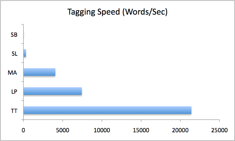
Table 2: Speeds

Words tagged per CPU second. Higher is better.

*If the dubious Joyce result is excluded, the average speed rises to 11.4 words per second. I’ve used this higher value in the speed comparisons below.

Table 3: Speed ratios

Ratio of words tagged per CPU second. Read as: Column entry over row entry, e.g., TreeTagger is 2.9 times faster than Lingpipe. Tagging speed in words per second added for reference.

Note that I’ve used the “by directory” speeds for Lingpipe and MorphAdorner, and excluded the possibly anomalous Joyce result from the Stanford bidirectional speed.

All of this in graphical form:

Discussion

The TreeTagger, Lingpipe, and Morphadorner taggers are all very fast; they process entire novels in seconds. Their speed is pretty consistent, too, though this fact is hidden a bit in the case of MorphAdorner by its significant startup overhead (20-30 seconds). Looking at MorphAdorner’s speed over the entire testing directory, rather than file by file, gives not only a much higher average speed (4000 wps vs. 1300) but much more consistent speed results (not shown in the tables above).

[Update: As noted above, cf. Bob Carpenter’s comment below for some notes on speed.]

These taggers tend to be slowest on the shortest works, especially Conrad, probably because there’s a fixed amount of overhead to start up a Java instance and perform another initialization steps, and Conrad’s novel is short enough for that to be a significant amount of the total processing time. This isn’t an issue in runs over an entire directory, where there’s only one startup instance, rather than file by file, and the overhead penalty in that case drops to zero as the corpus size becomes arbitrarily large.

Both Lingpipe and TreeTagger have the option to produce probabilistic results, that is, to produce output that includes several candidate parts of speech and the probability that each is correct for a given token. In Lingpipe, there’s a moderate penalty for doing so, somewhere around doubling the run time; in TreeTagger, the penalty is almost vanishingly small, around 10%.

Stanford’s tagger is much slower, working through novels in minutes or hours, depending on the analytical model used. There’s more variation in speed, too; the left3 model shows about a 4x difference between Joyce (slow) and Defoe (fast). Even excluding Joyce, which is something of an outlier, there’s a 2.6x difference between Melville and Defoe. The bidirectional model is similarly variable, especially if the Joyce result is correct. There’s a 10x spread between fastest and slowest results, or about 4x excluding Joyce.

The difference in tagging speed on Joyce in particular is interesting to me. Ulysses is surely the strangest and least conventionally grammatical of the bunch, and it doesn’t entirely surprise me that it should take longer to tag than the others. In fact I’m a bit suspicious of the fact that the other taggers not only don’t take longer to process it, but in some cases actually chew through it faster than any other text. Are they just throwing up their metaphorical hands and labeling a bunch of stuff junk? But I may be anthropomorphizing the algorithms. Just because I would find it hard to sort out Joyce doesn’t necessarily mean it’s especially hard to compute. Will look at this in the next post, on accuracy.

Comparing the taggers and models by speed, the TreeTagger, Lingpipe and MorphAdorner packages are all within an order of magnitude of one another. They are in turn one to two orders of magnitude faster than Stanford left3 and hundreds to thousands of times faster than Stanford bidirectional. Stanford left3 is about 30 times faster than Stanford bidi.

Conclusions

Everything here is provisional until I look at accuracy, obviously.

First, note that speed is a threshold property, as far as I’m concerned. Faster is better, but the question isn’t really “which tagger is fastest?” but “is it fast enough to do x” or “how can I use this tagger, given its speed?” I think there are three potentially relevant thresholds:

1. As a practical matter, can I run it once over the entire corpus?
2. Could I retag the corpus more or less on whim, if it were necessary or useful?
3. Could I retag the corpus in real time, on demand, if there turned out to be a reason to do so?

The first question is the most important one: I definitely have to be able to tag the entire corpus once. The others would be nice, especially #2, but I don’t yet have a compelling reason to require them.

With that in mind, there would have to be a pretty analytically significant difference in output quality to justify using the Stanford bidirectional tagger. Some quick calculations: Gutenberg has probably around 2500 usable English-language novels. Say they average 150,000 words each. Both of these are conservative estimates. That would mean 375 million words to tag. Assume, generously, that Stanford bidi averages 12 words per second. So a year of CPU time to tag the corpus. That could be cut down to something manageable with multiple, faster machines, but still, unless I get serious compute time, it would probably take a month or two. In principle, you only need to tag the dataset once, so this might be acceptable if it really did improve the analysis, but options 2 and 3 above would definitely be out with the bidi model, barring a major change in the amount of computing power at my disposal.

Also: The system requirements of the bidirectional model may be significant. As noted in passing above, giving Java a gig of RAM wasn’t enough for the Joyce and Eliot texts, which crashed out with insufficient memory at 43% and 93% complete, respectively. They’re too bloody slow to retest at the moment with 1.5 GB allocated. In any case, I couldn’t currently go above that, since I only have 2 gigs in the system. True, memory is cheap(ish), but it’s neither free nor infinite. A related point to investigate if necessary: Would more memory or other tweaks significantly improve speed with either of the the Stanford models?

The non-Stanford taggers could tag the entire corpus in a CPU day or less, and perhaps as little as an hour or two of real time with a small cluster. That would allow a lot of flexibility to rerun and to test things out. Stanford’s left3 model would take about two CPU weeks. That’s not ideal, but it’s certainly a possibility.

None of the taggers looks fast enough to do real-time reprocessing of the entire corpus given current computational power, but they could easily retag subsections in seconds to minutes, depending on size.

Finally, a brief foretaste on accuracy: Stanford’s own cross-validation indicates that the bidirectional model is 97.18% accurate, while left3 is 96.97%. It’s hard to imagine that 0.21% difference being significant, especially when both models drop to around 90% on unknown words. Haven’t yet seen or run similar tests on the others, nor have I done my own with Stanford. There’s reason to believe that MorphAdorner will be especially good on my corpus, given its literary training set, but that has yet to be verified; training other taggers on MorphAdorner’s data might also be possible.

Takeaway points on speed

Provisionally, then: MorphAdorner is probably the frontrunner: It’s fast enough, free, under current development, and geared toward literature. TreeTagger is fastest, but not by a qualitative margin. I’m also concerned that it’s not currently being developed and that the source code doesn’t appear to be available. Lingpipe is plenty fast, though I have some concerns about the license. Stanford left3 remains viable, but speed is a moderate strike against it. Stanford bidirectional is likely out of the running.

Here’s a quick summary of the POS taggers I’m looking at. This probably should have come before the initial results, but at the time there were only two candidates. Now it’s four. I’ll add others if I have a need or if people ask me to, but for the moment I’m satisfied with this list.

Lingpipe

As noted in an earlier post, Lingpipe is a commercial product from Alias-i. It’s a suite of Java applications for natural language processing, and it’s released under an unusual quasi-open-source license. If I’m reading the license correctly, you can use the software for free so long as you make the output freely available and aren’t selling whatever it is you do with it. My guess is that my research would qualify on all fronts, but I worry a bit about how the output redistribution requirement might limit my ability to work with commercial text repositories.

The version I’m evaluating is 3.6.0, which is current as of early November, 2008. It’s trained on the Brown corpus, which is made up of about a million words of American English published in 1961. There’s some fiction in the training set, but it’s a general-purpose corpus, not a literature-specific one. Lingpipe uses the what I presume is the Brown tagset (compare Alias-i’s own list of tags) and produces XML output. It can accept XML, HTML, or plain text input. It uses a hidden Markov model for POS determination, though I’m in no way equipped to know if that’s a good, bad, or indifferent thing.

Note: NLTK, to which Lingpipe sometimes refers, would be another option to check out if necessary. It’s written in Python and is just barely enough of a pain to install that I haven’t yet bothered. A review on the Linguist list had generally high praise for it as a teaching tool, but also said it was slower and less feature-rich than other packages. (“Many of the features that make it so good for learning get in the way of its usefulness for real work. … [NLTK is] too slow for programs involving large amounts of data.”)

Stanford

The Stanford POS tagger is part of the Stanford NLP group‘s suite of Java-based NLP tools. It’s licensed under GPL v.2, i.e., it’s free software. W00t!

I’m evaluating version 1.6, released 28 September 2008. The tagger is trained on a corpus from the Wall Street Journal (38 million words from 1988-89). It uses the Penn tagset (which is smaller than Brown, although that’s not necessarily a bad thing) and implements a maximum entropy tagging algorithm (ditto above on my inability to judge the relative merits of this approach). Takes plain text and XML input, produces equivalent output. The tagger offers two tagging models, left3words and bidirectional; the latter is said to be slower, but very slightly more accurate.

TreeTagger

TreeTagger is a project of the Institute for Computational Linguistics at the University of Stuttgart. It’s released under a free, non-commercial license. The software was developed in the mid ’90s and doesn’t look to be currently maintained, though I could be wrong about that. There’s also no source code obviously available; the package is distributed as precompiled binaries for Linux, Mac, and Windows. This isn’t an immediate problem, but it might limit future flexibility. I also haven’t looked especially hard for the source code, nor have I attempted to contact the project developers.

I’m working with version 3.2, using the English chunker and parameters v. 3.1, all of which are the current releases. TreeTagger uses a probabilistic decision tree algorithm that the author claims is slightly better than Markov models. It uses the Penn tagset and is trained on the Penn treebank, a 4.5+ million word combination of the WSJ, Brown, ATIS, and Switchboard corpora. XML/SGML and plain text input is supported, but output is plain text only. It can be configured to produce either the single best tag for each word, or to list multiple possibilities and their respective probabilities. Lingpipe can do something similar; Stanford cannot, I think.

MorphAdorner

MorphAdorner is produced at Northwestern and is part of the MONK project. The software hasn’t been formally released yet, but should be soon as the project draws to a close. The license is GPL v.2+.

MorphAdorner is designed to prepare texts for analysis within the larger framework of tools available in MONK. What’s especially cool, for my purposes, is that it’s trained on specifically literary corpora, down to the level of separate nineteenth-century American and nineteenth-century British fiction collections, plus early modern English. So it’s likely to be significantly more accurate out of the box than the others. (Note for further investigation: How much work would be involved in using MorphAdorner’s training sets with the other packages, if necessary?) It also uses a custom tagset that’s “designed to accommodate written English from Chaucer on within one descriptive framework” (Martin Mueller, pers. comm.) and is generally equipped to work with literary texts in many genres from middle English to the present, all of which distinguishes it from the other tools, which were generally developed for and by corpus linguists.

I’m evaluating a prerelease snapshot (labeled version 0.81) supplied to me by the developers on 6 November 2008. MorphAdorner is a commandline Java package, like Lingpipe and the Stanford tagger. It can handle XML or plain text input and produces equivalent output. (It would also be possible to write a new output routine to produce XML output from plain text input.) It uses a hidden Markov model, or so I infer from the Java class names (Pib, correct me if I’m wrong).

Next up …

I think that’s it for the descriptive bit. An update to the speed comparison post (to finish the Stanford bidirectional run and add TreeTagger and MorphAdorner results) is coming shortly.

This is the first in a short series of posts comparing part-of-speech taggers (at the moment, just Lingpipe and the Stanford NLP group’s tagger). I need to settle on one for my history and genre project, but/and I haven’t yet come across any kind of broad consensus concerning their relative merits. Note to self: Talk to the people over in linguistics.

So … this post is a description of the testing archive. I picked fourteen novels from Gutenberg; there’s nothing all that special about them, except that they’re fairly canonical (I’ve read all of them, which could be useful) and they feel more or less representative of English-language fiction in Gutenberg. (No strong claims on this front; a full characterization of Gutenberg will be part of the project proper.) They’re typical in length and are distributed reasonably well by British/US origin, author gender, and date of composition. The list, arranged chronologically:

• Defoe, Robinson Crusoe (1719), Gutenberg etext #521, 121,515 words. M/Brit.
• Richardson, Pamela (1740), #6124, 221,252 words. M/Brit.
• Austen, Sense and Sensibility (1811), #161, 118,572 words. F/Brit.
• Scott, Ivanhoe (1819), #82, 183,104 words. M/Scottish.
• Brontë, Jane Eyre (1847), #1260, 185,455 words. F/Brit.
• Hawthorne, The Scarlet Letter (1850), #33, 82,912 words. M/Amer.
• Melville, Moby-Dick (1851), #2489, 212,467 words. M/Amer.
• Stowe, Uncle Tom’s Cabin (1852), #203, 180,554 words. F/Amer.
• Dickens, Great Expectations (1861), #1400, 184,425 words. M/Brit.
• Alcott, Little Women (1868/1869), #514, 185,890 words. F/Amer.
• Eliot, Middlemarch (1871-72/1874), #145, 316,158 words. F/Brit.
• Twain, Huckleberry Finn (1885), 76, 110,294 words. M/Amer.
• Conrad, Heart of Darkness (1899/1902), 526, 38,109 words. M/Brit/Polish.
• Joyce, Ulysses (1922), #4300, 264,965 words. M/Irish.

A few observations on the archive:

• Size: 14 novels, 2.4 million words. This is a tiny fraction of the Gutenberg fiction holdings in English; there’s no way it can be fully representative, and I don’t claim otherwise. I’ve assembled it for benchmarking purposes only. Still, my hope is that it’s not radically unrepresentative.
• Distribution:
  • 9 men, 5 women
  • 9 British Isles (including Conrad), 5 American
  • 2 18th century, 10 19th, 2 20th
  • Maybe more to the point, genres/periods include the early novel, epistolary novel, realism (heavily represented), Romanticism, allegory, and early and high modernism.
• There’s a heavy skew toward men, Brits, and the nineteenth century. My guess is that this is true of the Gutenberg holdings overall; it’s also not hugely out of line with, say, the MONK project’s fiction archive. Actual numbers for Gutenberg as a whole will follow at some point in the future.
• Middlemarch is the longest text by a fair margin; Heart of Darkness is an outlier at an order of magnitude shorter. There’s an uncanny cluster of lengths around 185,000 words. I assume this has much to do with the economics of book publishing in nineteenth-century Britain. Will be interesting to see if this is true in the full holdings.

My preparation of the texts was minimal and pretty loose—again, the goal is benchmarking, not final critical accuracy. The files are all plain ASCII text. I removed the Gutenberg headers and legal disclaimers, as well as any critical apparatus (pretty rare in Gutenberg to begin with) and editor’s introductions. Chapter heads, prefaces by the original author, etc. stayed in. An archive of the prepared texts is available (tar.gz, 5 MB), though there’s no reason to get them from me rather than from Gutenberg unless you want to repeat my trials.

More shortly in two posts, one on speed and the other on statistics and accuracy.